EliashMEM
What is it?
EliashMEM
is a program to extract the Eliashberg function directly from the
photoemission data. Basically,
it takes input from the high
resolution
photoemission measurement, and unfolds the Eliashberg function for the
electron-phonon (or other bosonic modes) coupling by fitting to the
quasi-particle dispersion. The Maximum Entropy Method (MEM)
is employed to overcome the numerical instability for a direct
inversion.
This work is a collaborative effort involving researchers from a number of institutions: Junren Shi (Oak Ridge National Lab), S.-J. Tang (University of Tennessee), Biao Wu (University of Texas at Austin and ORNL), P.T. Sprunger (Louisiana State University), W. L. Yang, V. Brouet (Stanford University and Advanced Light Source of LNBL), X. J. Zhou (Stanford University), Z. Hussain (Advanced Light Source), Z.-X. Shen (Stanford University), Zhenyu Zhang and E. W. Plummer (University of Tennessee and ORNL).
The details of the technique can be found in Phys. Rev. Lett. 92, 186401 (2004). These slides provide an overview to the technique.
The related paper:
"Identification of Multiple Fine Structures in Electron Self-Energy of La2-xSrxCuO4,'' X. J. Zhou, Junren Shi, T. Yoshida, T. Cuk, W.L. Yang, V. Brouet, J. Nakamura, N. Mannella, S. Komiya, Y. Ando, F. Zhou, W. X. Ti, J. W. Xiong, Z. X. Zhao, T. Sasagawa, T. Kakeshita, H. Eisaki, S. Uchida, A. Fujimori, Zhenyu Zhang, E. W. Plummer, R. B. Laughlin, Z. Hussain, and Z.-X. Shen, submitted to Phys. Rev. Lett.
Installation
The source can be downloaded here.To compile, it needs a Fortran 77 compiler as well as two numerical libraries: Lapack and Blas.
To install, first unpack the package:
tar xvzf MEM.tgz
then edit Makefile
to accommodate the settings of your system, and typemake
to
build. The executable is called MEM3.
The examples directory includes a sample data set (dispersion.txt), which happens to be the data presented in the PRL paper, and the corresponding configuration file (CONF3.INI). To analysis the data, run the command in the examples directory:
The program reads input from a couple of input files and generate results to a number of output files.
The second input file is CONF3.INI. It contains various parameters controlling the behavior of the program (the essential parameters are denoted by red row numbers):
The working environment should include a easy-to use plotting software, e.g. gnuplot for Linux or Unix-like systems, so that the fitting quality can be constantly monitored.
It is distributed under the terms of the GNU General Public License (GPL).
The examples directory includes a sample data set (dispersion.txt), which happens to be the data presented in the PRL paper, and the corresponding configuration file (CONF3.INI). To analysis the data, run the command in the examples directory:
../MEM3
Usage
The program reads input from a couple of input files and generate results to a number of output files.
Input:
The program reads two input files. First is the dispersion data file from the experimental measurement. It is in simple text format with two columns: first column is the initial state energy in the unit of eV; the second column is the momentum in arbitrary unit. Note that the program only utilizes the data with energy below the Fermi energy.The second input file is CONF3.INI. It contains various parameters controlling the behavior of the program (the essential parameters are denoted by red row numbers):
| Row |
Field
name |
Explanation |
| 1 |
Data
File Name |
The
filename of the
input dispersion data |
| 2 |
Model
File Name |
The
program may be supplied with a constraint function. The file
is in simple
text format with first column being the photon energy
(ω) in
meV
and second column being the constraint function
m(ω).
The total number of rows should be NA. If it is set to
"NONE", the program uses the
simple constraint function described in the paper. |
| 3 |
Output
Prefix |
The
prefix for the output files. For instance, setting the field
to "Be1010", the output files will be "Be1010_SPT.dat",
"Be1010_DAT.dat" ... |
| 4 |
NDRAW |
The
total number of rows of the input dispersion data file |
| 5 |
NA |
The
total number of interpolation points for the output
Eliashberg function. If the constraint function is provided,
it should be the total number of rows of that file. |
| 6 |
Ecutoff |
The
high energy tail of the dispersion data is usually too noisy.
This parameter supplies a cutoff energy (in eV) and only the data
points below this energy
are utilized in the MEM fitting. |
| 7 |
KT |
Temperature
in Kelvin |
| 8 |
FITBPD |
Currently
not used. Always set it to zero. |
| 9 |
A1 |
The
bare particle dispersion is modeled as: ε0(k)=A1(k-kF)+A2(k-kF)2.
This is the first parameter. |
| 10 |
A2 |
Another
parameter for the bare particle dispersion. |
| 11 |
EF |
The
position of the Fermi energy (in eV). |
| 12 |
KF |
The
position of the
Fermi wave vector, in arbitrary unit. |
| 13 |
ERRB0 | Controlling
how the error bars of the real part of self-energy data (σi)
are determined:
|
| 14 |
ERRB1 |
Another
parameter for
the error bar determination |
| 15 |
Method |
Selecting
the MEM
algorithm:
|
| 16 |
Iternum |
The
maximum iteration
number for the MEM fitting. 1000 is usually
sufficient. In rare cases when the fitting is not converging,
set it to a larger number. (A non-converging MEM fitting will
give rise a Eliashberg with lot of artifacts). |
| 17 |
Alpha |
Depending
on the setting
of Method parameter:
|
| 18 |
DAlpha |
Only
referred when using
the Bryan's method (Method=3): step length for the iteration
of a. |
| 19 |
XCHI |
Referred
only when using the
historic method (Method=1): the target χ2 |
| 20 |
OmegaD |
The
parameter for the
constraint function (See Eq. 6 of the
paper): ωD |
| 21 |
OmegaM |
Another
parameter for
the constraint function: ωm.
It also set the maximum photon frequency above which the Eliashberg
function vanishes. |
| 22 |
M0 |
Another parameter for the constraint function: m0 |
| 23 |
Beta |
The
exponent for
calculating the average <ωβ> |
| 24 |
NBin |
This
divides the ω-axis to a NBin bins and the program calculates
<ωβ>
for each bin. It is followed by NBin+1 numbers that specify start and end points of each bin. |
Output
The screen output:
- ND: the number of data points utilized in the MEM fitting
- SIGMABAR: the average error bar of the real part of self-energy
- CHI^2: the mean deviation of the final fitting: χ2
- ALPHA: final value of a.
- LAMBDA: the mass enhancement
factor calculated
- DLAMBDA: error bar of the determined mass enhancement factor
- OMEGALOG: the average phonon frequency that appears in Eliashberg's Tc formula.
Output Files:
All output files start with [Output Prefix] that is supplied in CONF3.INI file:- [Output Prefix].LOG: includes various information for the fitting.
- [Output Prefix]_SPT.dat: the Eliashberg function: column 1: ω (meV); 2: Eliashberg function; 3: constraint function
- [Output Prefix]_DAT.dat: Self energy data and fitting. column 1: initial state energy (meV); 2: real part of self energy data (meV); 3: error bars (meV); 4: fitting to the real part of self-energy (meV); 5: calculated imaginary part of self-energy (meV).
- [Output_Prefix]_DSP.dat:
Dispersion data and
fitting: column 1: initial state energy data (eV); 2: momentum data; 3:
fitting to
the momentum data; 4: calculated
imaginary part of self-energy (eV); 5: calculated photoemission peak
width (FWHM).
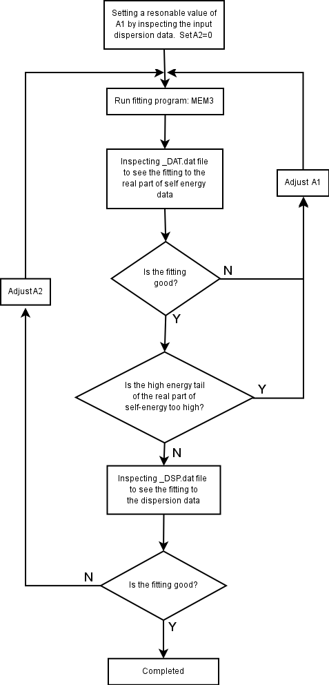
Working Flow
Unfortunately, the program is not fully automated. It still needs inputs of human being to get proper settings of parameters. The most important parameters are A0 and A1, which determine the bare particle dispersion through ε0(k)=A1(k-kF)+A2(k-kF)2. Fortunately, it is not too difficult to get a reasonable set of values for them by following the proper working procedure. It is hopeful the procedure will be automated in the future.The working environment should include a easy-to use plotting software, e.g. gnuplot for Linux or Unix-like systems, so that the fitting quality can be constantly monitored.
Issues and Comments
Please contact me (junrenshi@gmail.com) for questions, comments and suggestions.License
This program is released in hopes that it will be useful for other researchers. We can not be responsible for any consequence incurred by this program, neither will we claim credit for the results obtained from this program.It is distributed under the terms of the GNU General Public License (GPL).